Limitation: Requirement for Large Datasets
Table S1. Specific number of positive and negative samples for CVs
| Dataset (remain) | Y_train0 | Y_train1 | Y_test0 | Y_test1 | |
| 80% | 56981 | 15618 | 14245 | 3905 | |
| 64% | 45584 | 12495 | 11396 | 3124 | |
| 51.2% | 36478 | 9985 | 9120 | 2496 | |
| 20% | 14320 | 3836 | 3580 | 959 | |
| 4% | 2869 | 762 | 718 | 190 | |
| DDI2013* | 2792 | 510 | 699 | 127 |
* The number of remaining relationship pairs in the DDI2013 dataset after filtering and alignment.
The performance of the small dataset of DDI2013 is relatively poor compared to the large datasets of Ddinter and Drugbank. Therefore, we hope to continue to explore whether our method has high requirements for the dataset. We have added the following experiments
We randomly deleted relationship pairs from Ddinter based on the ratio of positive and negative samples to ensure sufficient samples for each training session. Afterwards, we conducted a 5-fold cross-validation on the new dataset and recorded the AUC and AUPR values. The specific number of positive and negative samples for cross-validations is shown in Table S1. The results obtained are presented in Figure S1 and Figure S2.
As illustrated in the figure, when we randomly decrease the number of positive and negative samples involved in training, regardless of the specific reduction amount, it is evident that our prediction metrics, AUC and AUPR, continuously decline. Notably, when more than 80% of the data is removed, there is a steep drop in both AUC and AUPR.
When we delete 96% of the data, we are left with 2869 entries labeled as 0 and 762 entries labeled as 1. The remaining test set contains 718 entries labeled as 0 and 190 entries labeled as 1. It can be observed that when the original dataset is reduced to only 4% (roughly the same number of relationship pairs as the DDI2013 dataset), the model’s performance deteriorates, with the AUC dropping to 0.742 and the AUPR decreasing to 0.452. This indicates that our method requires a large and accurate dataset to support its performance, which means, the quantity and quality of training samples have a significant impact on model performance. Reducing the dataset size, especially to a large extent, severely affects the model’s ability to generalize and make accurate predictions
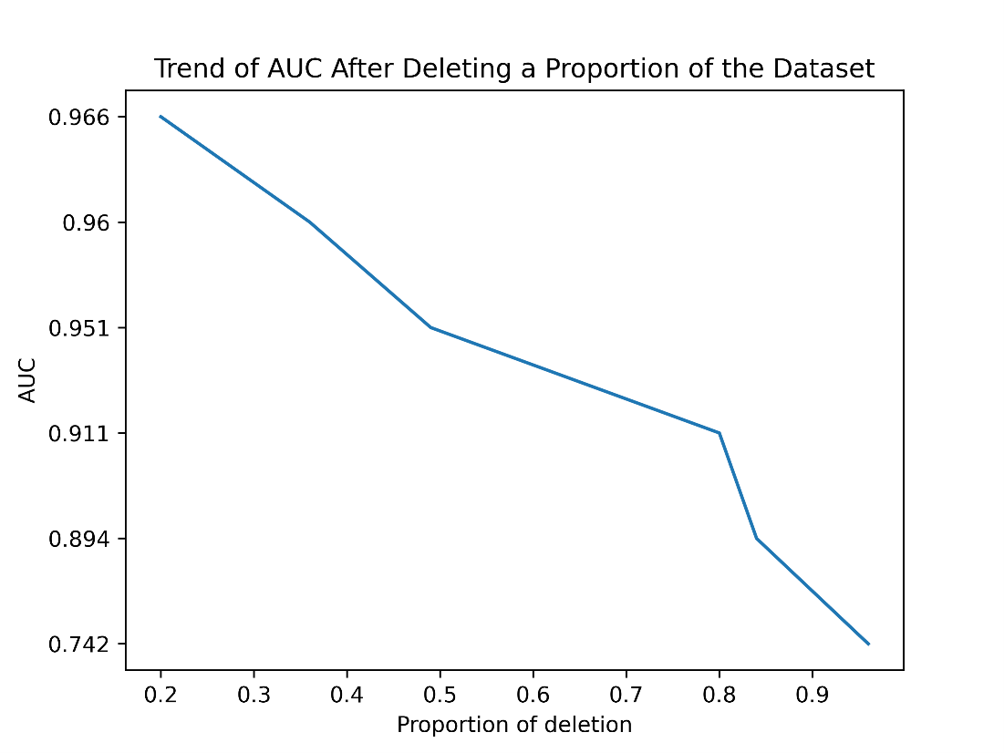 |
| Figure S1. Trend of AUC After Deleting a Proportion of the Dataset. When we randomly decrease the number of positive and negative samples involved in training, regardless of the specific reduction amount, it is evident that AUC continuously declines. |
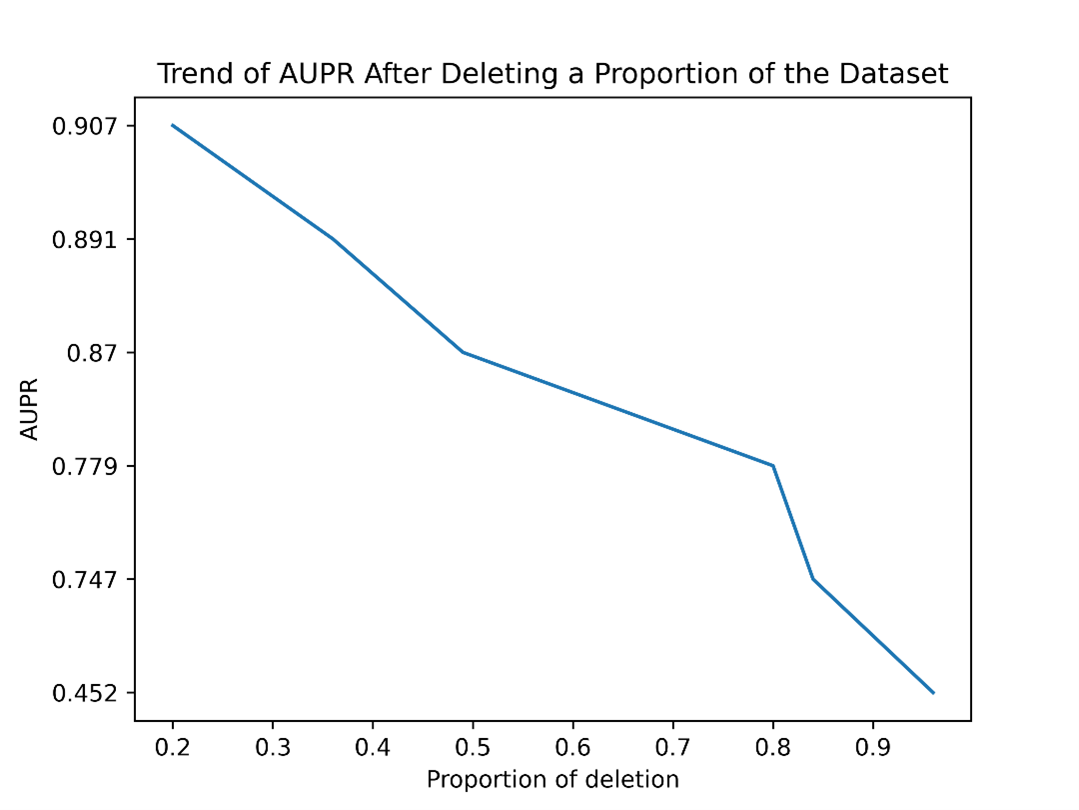 |
| Figure S2. Trend of AUPR After Deleting a Proportion of the Dataset. When we randomly decrease the number of positive and negative samples involved in training, regardless of the specific reduction amount, it is evident that AUPR continuously declines. |
Limitation 2: The storage space and computing power requirements of the dataset constructed using the splicing method will be further increased
Table S2. Details of each dataset
| Dataset | Balanced | Sampling | DD-Type | Positive | Negative | File_size |
| DDI2013 | No | No | DDI | 637 | 3491 | 0.12GB |
| DrugBank | Yes | Yes | DDI | 191808 | 191808 | 11.57 GB |
| DDinter | No | No | DD intensity (Major? or not) | 24647 | 90311 | 3.43GB |
If there are high requirements for the size of the dataset, what we need to further explore is whether further expansion will lead to the need for particularly large storage space and computing power.
Our method involves concatenating features, so as the dataset expands, more storage and computing resources will be required to scale up the training.
For instance, Table S2 shows that DDI2013 contains 4,128 relationship pairs and occupies 0.12GB, while DrugBank has 383,616 pairs and occupies 11.57GB. The dataset expanded by 92.93 times, but the storage increased by 96.42 times.
Therefore, it can be inferred that as the dataset grows, the storage demand will further increase. Currently, our algorithm runs on a GTX4080 platform with 12GB memory, an i9-13900HX processor, and 64GB DDR4 RAM. For larger datasets, more advanced hardware will be needed.
Imbalanced issue
To address the issue of the imbalanced dataset, we designed another experiment. Currently, in our dataset, the number of positive samples (major) is much smaller than the number of negative samples (moderate, minor). Since it is difficult to introduce relationships using oversampling methods (no other datasets contain information on drug-drug interactions), we opted for a down sampling method (i.e., randomly deleting some negative samples). This resulted in a balanced dataset, DS1, and two other imbalanced datasets, DS05 and DS2. In DS1, the number of negative samples is equal to the number of positive samples; in DS05, the number of negative samples is half that of the positive samples; and in DS2, the number of negative samples is double that of the positive samples.
Table S3. Down-sampling results
| Dataset | AUC(mean) | Std (AUC.) | AUPR(mean) | Std (AUC.) |
| DS05 | 0.9455 | 0.0026 | 0.967 | 0.0026 |
| DS1 | 0.9577 | 0.0015 | 0.9543 | 0.0023 |
| DS2 | 0.9657 | 0.0011 | 0.9371 | 0.0024 |
| DS_original | 0.9704 | 0.0011 | 0.9198 | 0.003 |
Set label “major” as label ‘One’ issue
Secondly, our case study on the drugs in the dataset that were not involved in training shows that using this method for modeling and prediction yields excellent results.
Thirdly, our approach is more inclined to identify stronger relationships in drug-drug interactions. An intuitive hypothesis is that if we set major as 1 and the others as 0 during dataset design, it could better help us discover “strong” relationships.
To further validate our hypothesis, we designed a new experiment. First, we randomly selected 5,000 major relationship pairs from the dataset (and removed them from the training set) to create an independent dataset. Next, we trained the model using Major as label1, and then using both major and moderate as label1, with the rest set as label0.
Subsequently, we randomly selected 5,000 drug-drug relationship pairs as a control group of negative samples. We then compared the average scores of the 5,000 major independent dataset with the 5,000 randomly selected negative samples. The results are shown in Table S4. When using the Major label as label1, the average score was lower, but it was more likely to classify the randomly selected negative samples as negative (resulting in a lower score). In contrast, when using the moderate label along with Major as label1, the average score was higher, but it also tended to assign higher scores to negative samples (leaning towards classifying randomly selected negative samples as positive).
We compared the difference in averages between the two approaches and found that using the major label as label1 resulted in a greater difference in average scores between the independent positive sample dataset and the randomly selected negative sample dataset. This indicates that this method allows the model to better identify strong DDI relationships.
Table S4. Independent dataset/ random selected negative samples results
| Label type | Independent (Positive mean) | Random selected (Negative mean) | Variance |
| Major(1) | 2.6593 | -5.4055 | 8.0647 |
| Ma+Moderate(1) | 5.8171 | 3.5836 | 2.23353 |
Other metrics
As DDintensity is a predict and rank model, our framework focuses on more threshold-less metrics, such as AUC and AUPR.
It usually needs a threshold to calculate the metric for accuracy, precision, and recall. Moreover, the threshold is critical as it may influence performance. However, to further evaluate our models, we calculated F1, Recall, and Precision. For reference, we set the threshold as the mean value of all predicted scores for each modality. As shown in table, S4, which records F1, Recall, and Precision. We can see that the embedding we used ranks first in F1, second in Recall, and first in Precision among all the embeddings involved in the comparison.
Table S5. Results comparisons with different embeddings
| Embeddings | F1 | F1_std | Recall | Recall_std | Precision | Pre_std |
| 3DResnet50 | 0.7312 | 0.0047 | 0.9422 | 0.0042 | 0.7069 | 0.0042 |
| DinoVitb16 | 0.727 | 0.0036 | 0.9504 | 0.0027 | 0.7088 | 0.0031 |
| GAT(DDI) | 0.6731 | 0.0047 | 0.944 | 0.0043 | 0.6834 | 0.0037 |
| Bart | 0.7633 | 0.005 | 0.9712 | 0.0025 | 0.7318 | 0.004 |
| SapBert | 0.76 | 0.004 | 0.9748 | 0.0023 | 0.7268 | 0.0035 |
| SMILEFIN | 0.7045 | 0.0046 | 0.9288 | 0.0046 | 0.6939 | 0.0038 |
| RDF2VEC | 0.76 | 0.0042 | 0.9801 | 0.0028 | 0.7254 | 0.0036 |
| SciBert | 0.7527 | 0.0036 | 0.9715 | 0.0023 | 0.7223 | 0.003 |
| GADNN | 0.6684 | 0.0069 | 0.9118 | 0.0074 | 0.6672 | 0.0059 |
| ChemBERTa-2 | 0.7293 | 0.0029 | 0.9593 | 0.0031 | 0.7124 | 0.0029 |
| bioGPT | 0.7704 | 0.0037 | 0.9761 | 0.0024 | 0.7367 | 0.0032 |